A Gentle Introduction to Token Embeddings

The journey of text, from Encodings to Embeddings

Have you ever trained a machine learning model for text classification or a recurrent neural network for language translation? Or maybe your own transformer model. All these tasks require you to somehow represent text information in numeric format. This need for this kind of representation is fundamental: None of the machine learning algorithms, including deep learning and GenAI algorithms understands words the way we understand them. All they understand is numbers: integers, floats and their combination (eg. vectors).

Hence, one of the most fundamental challenges is bridging the gap between human language and machine understanding. At the heart of this challenge lies a crucial concept: token embeddings.

But what exactly are token embeddings? How have they evolved over time? And why are they so critical to the success of today's advanced language models?

In this article, we'll embark on a journey through the landscape of token embeddings. We'll start with the classical approaches that paved the way, explore the revolutionary Word2Vec model, and finally delve into the sophisticated embedding techniques powering the latest transformer models.

Let’s start with a cliched example, I am at least 80% certain you have heard this sentence if you are in the journey of learning NLP:

The cat sits on a mat

In Human Minds like ours, we picturize a cat (Snowbell from Stuart Little movie, anyone?) sitting on a mat. (By giving the human mind reference, I have also subtly mentioned this article is written by a human.)

However, for our computer friends, the representation could be one of the many, as described below. All of them are useful in their own way.

1 Types of Word Representations

1.1 Bag-of-Words (BoW)

While this blog is about modern embeddings used in large language models, appreciating them is difficult without knowing their precursor.

Bag-of-Words is a long vector of mostly zeros and a few non-zeros, the length of the list being the number of words in the vocabulary. The non-zeros would be the frequency of the words, and would occupy the position corresponding to the words present in the sentence.

Let us consider we have a small corpus of text:

The cat sits on a mat
The dog sits on a mat
The mat is clean

The vocabulary size in this case is 9, and each sentence would be represented as in the screenshot below:

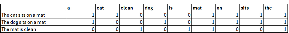
Each position in the vector corresponds to a word in the vocabulary. The value at each position indicates the frequency (or presence) of the corresponding word in the text.

Each word can also be represented as a vector, with a ‘1’ at the corresponding location in vocabulary. For example, the words ‘a’, ‘cat’, ‘clean’ and ‘the’ can be represented as below:

a:     [1, 0, 0, 0, 0, 0, 0, 0, 0]
cat:   [0, 1, 0, 0, 0, 0, 0, 0, 0]
clean: [0, 0, 1, 0, 0, 0, 0, 0, 0]
the:   [0, 0, 0, 0, 0, 0, 0, 0, 1]

1.2 TF-IDF Vectors

A vector similar to above, but the ones would be respectively replaced by numbers normalized by a factor of how frequently they occur in the document (sentence) and corpus.

Not going into details, but it is also a sparse representation. The zeros remain as they are, the ones are replaced by normalized values.

1.2.1 Problem with these embeddings

Given any two of these word vectors, what would their cosine similarity be? Since these vectors are sparse and high-dimensional, there is no shared context. Hence, cosine similarity between two words is 0. So while these techniques did a good job representing the sentence, the concept of semantic similarity was not a thing.

However, in 2013, the landscape of Natural Language Processing was going to be changed forever. The introduction of word embeddings by Mikolov’s group from Google would change the way we represent text data. The Word2Vec would eventually become the precursor of modern token embeddings.

1.2.2 Moment of Appreciation for the Classical Techniques

While the modern embeddings do solve the problems associated with ‘curse of dimensionality’ and ‘semantic similarity’, let us take a moment to appreciate their classical counterparts.

Of all the tests, one test they have passed is the test of time. Bag-of-words was introduced in 1950s, and almost 70 years later, as I am writing this blog in 2024, they are still not irrelevant. TF-IDF too has celebrated its golden jubilee, yet any introduction to NLP would not be complete without its mention. Not every algorithm has met this fate.

On a side note, when doing sentiment analysis, try using a Naive Bayes or a Logistic Regression model with TF-IDF embeddings. I have personally found their results outperforming the mighty BERT. Sometimes, old is indeed gold!

1.3 Comes Word2Vec

Word2Vec is a pivotal point where we move from sparse embeddings to dense. Here, words are represented as a dense vector with a length much less than the vocabulary (usually in the scale of a few hundreds). These are trained on very large corpuses of text data, typically tweets, news articles etc. The way to train these is out of scope of this blogpost, but there are mainly 2 ways to train them: Skip gram and Continuous Bag of Words (CBOW).

Since the embeddings are dense, they open pathways for kinds of interpretations we could not think using the techniques talked before. We can find how similar (or dissimilar) two words are in terms of their meaning, add two words or find distance between two words.

Here is a small example, implemented using popular Python library called gensim.

In the first example, let’s see how a word vector looks like:

The example uses a Word2Vec pretrained on google news data where vector for the word ‘lion’ is looked up. Turns out, it looks like just any random vector. Nothing fancy!

But things are getting to get more interesting now: They allow us to find how similar (or dissimilar) two words are. We can find the words in English dictionary that are most similar to the word ‘lion’.

And the word most similar to lion is lions (very insightful, isn’t it?)

In the example below, I see the similarity score for lion and tiger is higher than lion and zebra, indicating that a lion is more similar to a tiger (big cats).

The other kind of embeddings called GLoVe are similar too.

2 Modern Token Embeddings

How are very modern embeddings, like the ones used in transformers different from their older counterparts? The answer is they are trained at a sub-word level. The advantage of using sub-word is that out vocabulary size goes down drastically. Like OpenAI’s tiktoken library has vocabulary size of 50257 for English, which is much less than the size of English vocabulary.

Think about it, the smaller the size of subword is, the less size we need. If we drop down to simple alphabet level, we only need 26 + a few tokens to represent entire English language.

Any transformer implementation in PyTorch would have the code nn.Embedding(vocab_size, n_embed). Vocab_size represents how many tokens our tokenizer understands, and n_embed is the embedding dimension. Let’s see how this changes the way we represent our words.

The advantage of using a function like nn.Embedding() is that our dimensionality is now a dynamic feature, granting us the flexibility to experiment with multiple values. This is a game-changer in the world of embeddings. Moreover, it makes these embeddings trainable and hence dynamic, meaning that our embeddings will evolve and adapt according to the specific dataset and task at hand.

To put this in perspective, imagine training a model for sentiment analysis on movie reviews versus training one for medical text classification. With nn.Embedding(), the same architecture can learn different optimal representations for each task. This is unlike the static nature of Word2Vec embeddings which, once trained on a general corpus, remain constant regardless of the downstream task.

2.1 Dimensionality:

Whether at word level (Word2Vec) or subword level, higher dimensions (larger n_embed) allow for more information to be packed into each vector. This can lead to more nuanced representations of tokens, potentially capturing subtle differences in meaning or usage. However, there's a trade-off: more dimensions mean more parameters to train, which increases computational cost and the risk of overfitting.

On the flip side, lower dimensions are computationally efficient and can generalize well, but might miss out on some of the finer details of language.

In practice, the choice of embedding dimension often comes down to a balance between model performance and computational resources. Common values range from a few hundred to a few thousand, depending on the scale of the model.

The Word2Vec example we saw above uses 300 dimensions to capture a word, however can have higher or lower dimensions. In my experience transformers operate at a much larger dimensionality.

2.2 Embedding table

Now that we've touched on modern token embeddings, let's dive a bit deeper. At the core of these embeddings is what we call an "embedding table". Think of it as a giant lookup dictionary where each token (remember, these are now sub-word units) has a corresponding vector.

In code, when we see nn.Embedding(vocab_size, n_embed), we're essentially creating this table. vocab_size is how many unique tokens our model knows, while n_embed is the length of each token's vector.

2.3 Position Encoding

Remember our old friend, the Bag-of-Words model? One of its major drawbacks was that it completely ignored word order. "The cat sits on a mat" and "The mat sits on a cat" would have the same representation!

Modern transformer models solve this problem with positional embeddings. These are vectors that encode information about a token's position in the sequence.

This happens when we combine token embeddings with positional embeddings. Typically, this is done through simple addition:

Final Embedding = Token Embedding + Positional Embedding

This allows the model to understand both the meaning of a token (from its token embedding) and its context within the sequence (from its positional embedding).

3.0 Summary

We explored classical representations like Bag-of-Words and TF-IDF, which, while sparse, are still relevant for certain tasks like sentiment analysis. We also discussed modern dense embeddings like Word2Vec, GLoVe, and the sub-word embeddings used in transformers. Additionally, we highlighted the role of positional encodings in addressing word order issues.

Summarizing all the points we discussed in this post:

• Importance of word representations.

• Need for tokenization

• Classical word representation

  • Introduce sparsity and high dimensionality:

    • Bag of words

    • TF-IDF tokenization

  • Classical word representations are cannot tell similarity between any 2 words.

  • They are still useful on multiple fronts: like sentiment analysis.

• Word can be represented as vectors using techniques like Word2Vec and GLoVe.

  • Their dimensionality determines how much information and nuances they can carry.

  • They enable us to find similarities between two words using cosine similarity.

• Modern embeddings are extension to word embeddings.

  • They are calculated at a sub-word level.

  • They are flexible and dynamic.

  • We can use nn.Embedding() function inside of PyTorch to compute them dynamically. There is no need to pre-train them. However, we can also use pre-trained ones.

  • Positional encodings are added to token embeddings to identify the order of words.

4.0 References:

• HuggingFace, Cohere, OpenAI and other embeddings:

• https://huggingface.co/blog/getting-started-with-embeddings

• https://jalammar.github.io/illustrated-word2vec/

• https://radimrehurek.com/gensim/models/word2vec.html